Black-Scholes gives you a closed-form price for a vanilla European option in one line — so why bother simulating? Because the moment an option’s payoff depends on the path (Asian, lookback, barrier) or you add non-linearity (American exercise, Vol surfaces, XVA), the formulas stop existing and Monte Carlo keeps working.
In this post we build a complete Monte Carlo pricer from scratch in NumPy, verify it against Black-Scholes, then extend it to path-dependent payoffs and Greeks. Every number shown comes from a single run with a fixed seed (numpy.random.default_rng(42)) — you should be able to reproduce all of them.
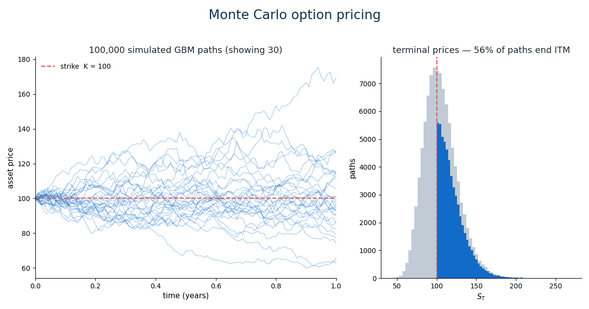
The model: geometric Brownian motion #
Under the risk-neutral measure the asset follows GBM:
dS/S = r·dt + σ·dW → S(t+dt) = S(t)·exp((r − σ²/2)·dt + σ·√dt·Z)The discretization is exact in log-space, which makes the simulation a one-liner with cumsum: draw the standard normals once as a matrix, and every path exists in memory before you price anything.
import numpy as np
from scipy.stats import norm

rng = np.random.default_rng(42)

S0, K, r, T, sigma = 100.0, 100.0, 0.05, 1.0, 0.20
n_steps, n_paths = 100, 100_000

dt = T / n_steps
Z = rng.standard_normal((n_paths, n_steps))
log_paths = (r - 0.5 * sigma**2) * dt + sigma * np.sqrt(dt) * Z

S = np.empty((n_paths, n_steps + 1))
S[:, 0] = S0
S[:, 1:] = S0 * np.exp(np.cumsum(log_paths, axis=1))
Price a European call — and verify it #
MC pricing is three steps: payoff → average → discount.
ST = S[:, -1]
df = np.exp(-r * T)
payoff = np.maximum(ST - K, 0)

mc = df * payoff.mean()
stderr = df * payoff.std(ddof=1) / np.sqrt(n_paths)
Then check it against the closed form:
d1 = (np.log(S0 / K) + (r + 0.5 * sigma**2) * T) / (sigma * np.sqrt(T))
d2 = d1 - sigma * np.sqrt(T)
bs = S0 * norm.cdf(d1) - K * np.exp(-r * T) * norm.cdf(d2)
Output from the run:
Black-Scholes reference: 10.4506
Plain MC:  10.4750  (95% CI ± 0.0915)
10.4506 sits comfortably inside the Monte Carlo confidence interval. Never report a simulator output without its standard error — SE = σ/√n shrinks with √n, so 100× more paths buys you only 10× tighter error bars.
Halve the error for free: antithetic variates #
Every GBM path is driven by normals Z. Average each payoff with the payoff of the path driven by −Z and payoffs average around a common mean — the two estimation errors partially cancel:
# Mirror ONLY the random part; keep the drift term exactly as-is
D = (r - 0.5 * sigma**2) * T                     # total drift over T
ST_anti = S0 * np.exp(2 * D - np.cumsum(log_paths, axis=1)[:, -1])

payoff_anti = 0.5 * (np.maximum(ST - K, 0) + np.maximum(ST_anti - K, 0))
mc_anti = df * payoff_anti.mean()
se_anti = df * payoff_anti.std(ddof=1) / np.sqrt(n_paths)
Plain MC: 10.4750 (95% CI ± 0.0915)
Antithetic MC: 10.4708 (95% CI ± 0.0458) ← 50% SE reduction, same 100,000 pathsWatch the classic bug here: mirror the noise −Z, not the whole log-path −L. I mirrored exp(−cumsum(log_paths)) on the first attempt and got $8.78 — silently biased, perfectly plausible-looking, and completely wrong. The drift term must stay +D in both members of the pair; only the Brownian part flips sign.
Path-dependent payoffs — where MC earns its keep #
Each of these is one line on top of the path matrix S:
# Asian (arithmetic average strike) — payoff on the mean of the path
asian = df * np.maximum(S.mean(axis=1) - K, 0).mean()

# Lookback — strike is the path maximum the holder "would have" seen
lookback = df * np.maximum(S.max(axis=1) - K, 0).mean()

# Up-and-out barrier at B = 120 — knocked out if the barrier is ever touched
B = 120.0
hit = (S >= B).any(axis=1)
barrier = df * np.where(hit, 0, np.maximum(ST - K, 0)).mean()
Asian option: 5.7481
Lookback option: 17.8882
Barrier (120 UO): 1.4197 (38.1% of paths knocked out)Three exotic prices from the same simulated path matrix. This is the real economy of Monte Carlo: simulate once, price many derivatives.
One subtlety worth knowing: discretely monitored barrier options are priced higher than continuously monitored ones (the barrier can be “jumped over” between grid points) — for exact continuous-monitoring prices you’d use Brownian-bridge correction. Our number is the discrete-monitoring price, which is what the code simulates.
Greeks from the same Z
#
Bump-and-reprice, but with common random numbers: reuse the identical Z matrix for the bumped and unbumped runs. Without it, finite-difference Greeks are pure noise at realistic bump sizes.
Z_fix = rng.standard_normal((n_paths, n_steps))    # one Z, reused everywhere below

def mc_price(S0_=S0, sigma_=sigma, Z=Z_fix):
    lp = (r - 0.5 * sigma_**2) * dt + sigma_ * np.sqrt(dt) * Z
    ST_ = S0_ * np.exp(np.cumsum(lp, axis=1))[:, -1]
    return df * np.maximum(ST_ - K, 0).mean()

h = 0.01
delta = (mc_price(S0_=(1 + h) * S0)     - mc_price(S0_=(1 - h) * S0))     / (2 * h * S0)
vega  = (mc_price(sigma_=(1 + h) * sigma) - mc_price(sigma_=(1 - h) * sigma)) / (2 * h * sigma)
Delta 0.6355 (Black-Scholes: 0.6368)
Vega 37.3712 (Black-Scholes: 37.5240)Both land within a hair of the closed form — the residual gap is finite-difference error plus MC error, and shrinking h further eventually just adds noise (another reason to always know your SE).
American options: LSM #
European-style payoff tricks don’t capture the right to exercise early. Longstaff–Schwartz (Least Squares Monte Carlo) approaches it by regressing the continuation value on the state at each time step, walking backwards:
from numpy.linalg import lstsq

def lsm_put(paths, strike, rate, maturity, steps):
    dt_ = maturity / steps
    cf = np.maximum(strike - paths[:, -1], 0.0)          # payoff at expiry
    t_cf = np.full(len(paths), steps, dtype=int)         # time index of each cashflow

    for t in range(steps - 1, 0, -1):
        itm = np.where(paths[:, t] < strike)[0]
        if len(itm) == 0:
            continue
        disc = np.exp(-rate * dt_ * (t_cf[itm] - t))     # discount each cashflow to time t
        Y = disc * cf[itm]
        s = paths[itm, t] / strike                       # normalized state → well-conditioned
        X = np.vstack([np.ones(len(itm)), s, s**2]).T
        beta = lstsq(X, Y, rcond=None)[0]
        continuation = beta[0] + beta[1] * s + beta[2] * s**2
        exercise = strike - paths[itm, t]
        early = continuation < exercise
        idx = itm[early]                                 # commit to early exercise
        cf[idx], t_cf[idx] = exercise[early], t

    return (np.exp(-rate * dt_ * t_cf) * cf).mean()
Compared to the naive “keep one values array” version you’ll find in older tutorials, tracking each path’s cashflow time (t_cf) matters: a path that skips several steps before exercising must be discounted from its actual exercise date, not by one step. Running it (200,000 paths, 100 steps):
European put (closed form): 5.5735
American put (LSM):         6.0581   ← early-exercise premium ≈ 0.48
Two honesty notes from practitioners: LSM gives a lower bound on the true American value (early exercise is under-detected through regression noise), and the regression basis / ITM filter matter more than people expect — the s = S/K normalization above isn’t cosmetic, it keeps the linear algebra well-conditioned.
Bonus: portfolio VaR for free #
The same simulator answers risk questions in one line (this is essentially the Monte Carlo VaR from the Basel/FRTB toolbox):
returns = rng.multivariate_normal(mean_returns, cov_matrix, 100_000)  # cross-asset shocks
portfolio_returns = returns @ weights
VaR_95 = -np.percentile(portfolio_returns, 5)
ES_95  = -portfolio_returns[portfolio_returns < np.percentile(portfolio_returns, 5)].mean()
ES (expected shortfall, the average loss beyond the VaR threshold) is what FRTB moved to for internal-models capital — VaR tells you where the tail starts, ES tells you how deep it goes.
What to remember #
- Simulate in log-space with
cumsum— vectorized, exact per step, one matrix holds every path - Always report SE (
± 1.96·σ/√n); error shrinks like√n, so precision is expensive — variance reduction is cheaper - Antithetic variates: mirror
−Z, keep the drift; ~50% SE cut here for free - Common random numbers for finite-difference Greeks — reuse the same
Z - Verify against a closed form whenever one exists — it’s the cheapest bug detector you have
- Discrete ≠ continuous monitoring for barriers; LSM gives a lower bound for Americans
References #
- Boyle, P. (1977). Options: A Monte Carlo Approach — the original
- Longstaff, F. & Schwartz, E. (2001). Valuing American Options by Simulation: A Simple Least-Squares Approach
- Glasserman, P. Monte Carlo Methods in Financial Engineering — Paul Glasserman [Amazon]
- Hull, J.C. Options, Futures, and Other Derivatives — John C. Hull [Amazon]